TQM 2022

---

Topological Quantum Matter 2022

> Welcome to the "Geometric optimization of non-equilibrium adiabatic thermal machines" poster's page :)

You can download a digital copy here. The poster is based on the publication PRXQuantum.3.010326.

>> You're probably @BA. Here are some (not so touristy) recommendations

Parrilla/Asado: El boliche de Darío, El Ferroviario (usually hard to find place, call first!), Don Zoilo, El Desnivel

True tango: Here you can find a daily list of "milongas": hoy-milonga. If you want to hear a great local Tango player go to Cátulo Tango and listen to the Esteban Morgado Quartet.

Buenos Aires is the best place to read Borges. You can find very cheap books at the used books fairs near Plaza Italia and Parque Rivadavia

Ice cream? Probably Scannapieco is one of the best.

>>> A small optimization game

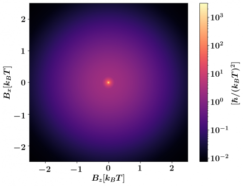
In Figure 3 you can see some lobe-like regions of big \(| \nabla_B \times \vec\Lambda(\vec B) |\). We easily see that a cycle enclosing one of these lobes will 'pump' a significant amount of heat (i.e. big \(A\)). Conversely, the value of \(\mathcal{L}^2\) for a given trajectory cannot be visualized so clearly since the dissipation is direction-dependent. However, a useful quantity to plot is the maximum eigenvalue of the symmetric tensor \(\underline \Lambda(\vec B)\). This value is an upper bound for the dissipation at each point of the parameter's space (and allows us to identify high-dissipative regions!). Below you can see a plot of the maximum eigenvalue of \(\underline \Lambda(\vec B)\):

From the above plot it is clear that protocols going near \(\vec B=0\) will likely dissipate a lot. Next, you can try to find an optimal trajectory for the power \(P\) of the qubit operating in engine mode. The sliders change the shape of quite generic elliptic trajectories, and you can choose to see \(\nabla_B \times \vec\Lambda(\vec B)\) or \(max.\lbrace eigenvalues[\underline \Lambda (\vec B)]\rbrace\). Use the green button to compute \((A/\mathcal{L})^2\). The best we could find was a value of \(\approx 0.031\).

>>>> References

[1] Bibek Bhandari, Pablo Terrén Alonso, Fabio Taddei, Felix von Oppen, Rosario Fazio, and Liliana Arrachea, Geometric properties of adiabatic quantum thermal machines, Phys. Rev. B 102, 155407 (2020).

[2] Also studied as the Cheeger problem, see Refs. [50-57] in the article.

[3] The value of \(\kappa\) is zero along the \(B_x\) and \(B_z\) axis (because the qubit decouples from one of the reservoirs). Take the limiting protocol with \(\Omega=\pi/2\) and \(R \rightarrow\infty\) for the curve (d) of Figure 4. You find \(x \rightarrow 0\) in Eq. (8), then \(\tau_\eta \rightarrow \infty\) and \(\eta \rightarrow \eta_C\), so it corresponds to the Carnot limit. The resulting value of \(A\) for this protocol (see Fig. 3) is \(A=\int_{\text{quadrant}} (\nabla_B \times \vec \Lambda) \cdot d\hat y = k_B T \log(2)\)... Why?